I. Intro
Date: 03/29/2023
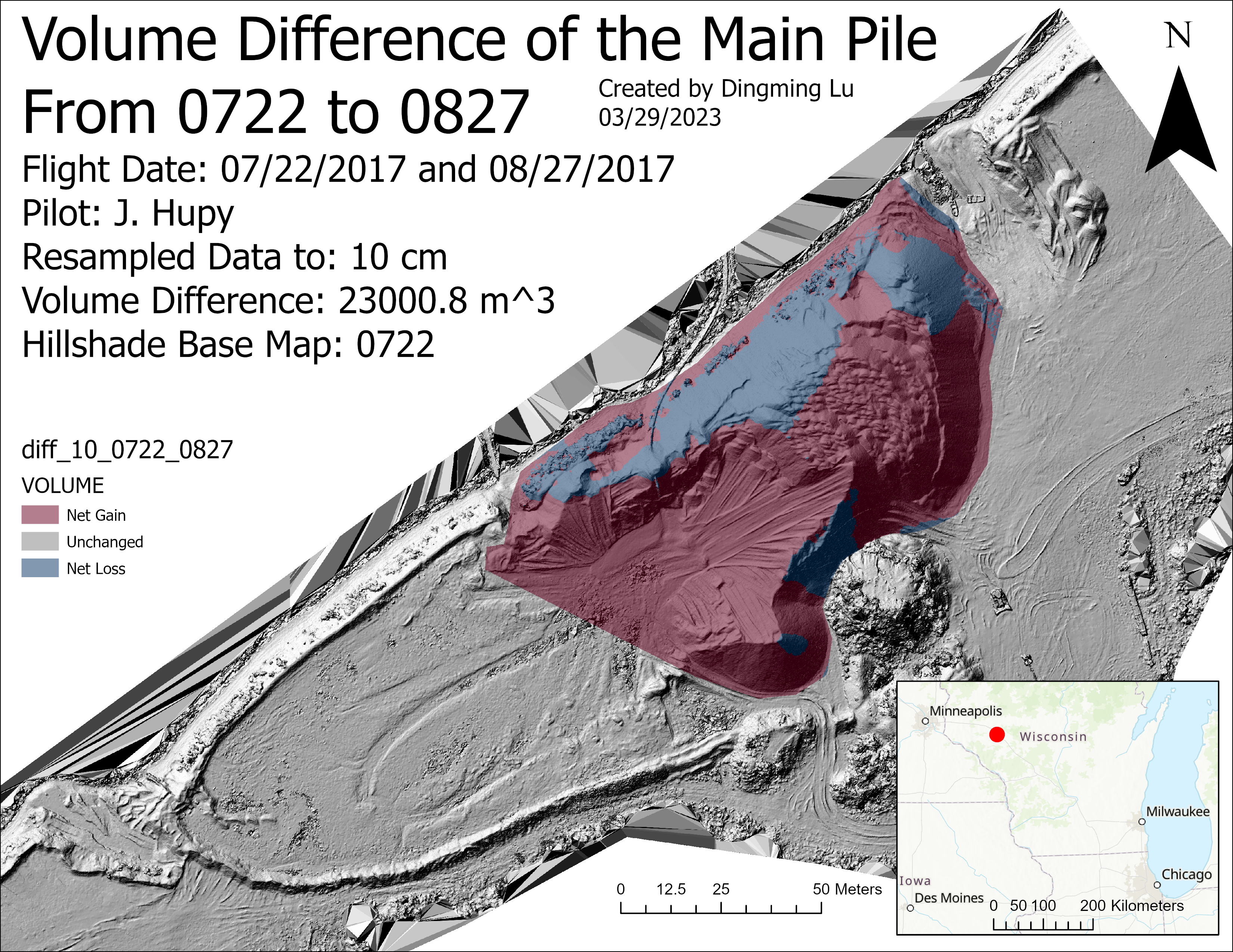
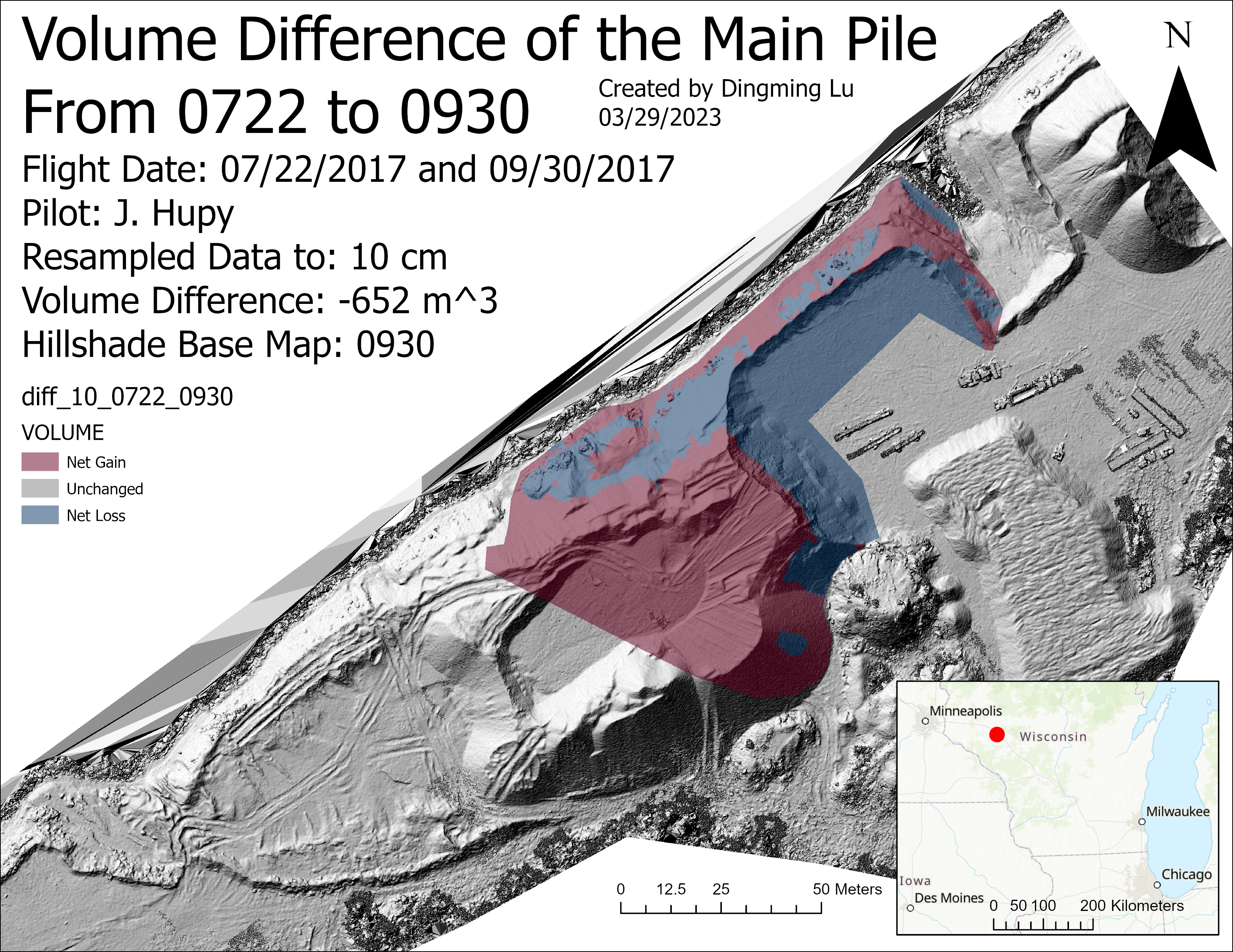
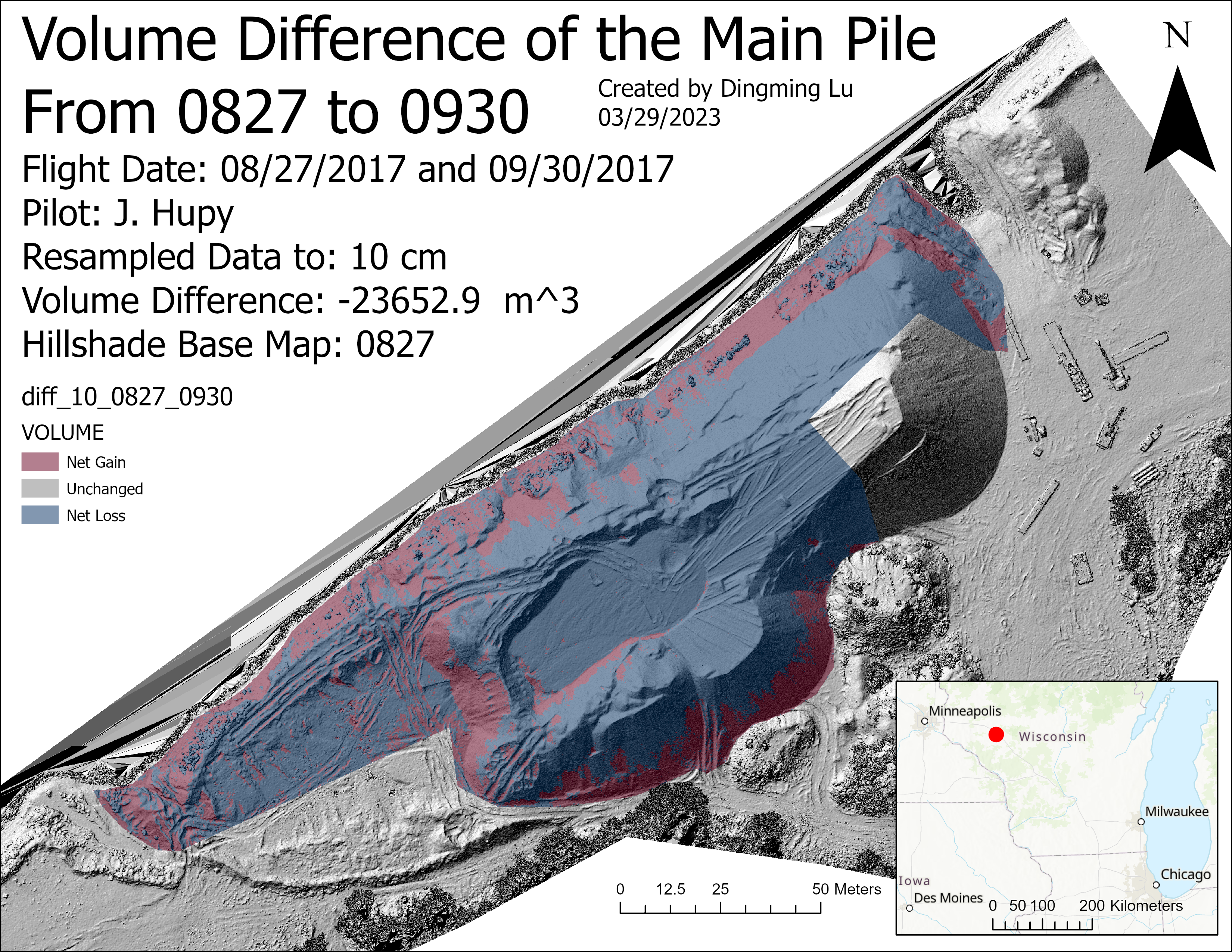
During the first lab, we worked with raster data. The first data was gathered at Wolfpaving. The second data was gathered by Prof. Hupy in 2017 for a real world case. Three flights were on July 22nd, August 27, and Steptember 30. 0722, 0827, and 0930 will be used for short.
II. Wolf Paving Analysis
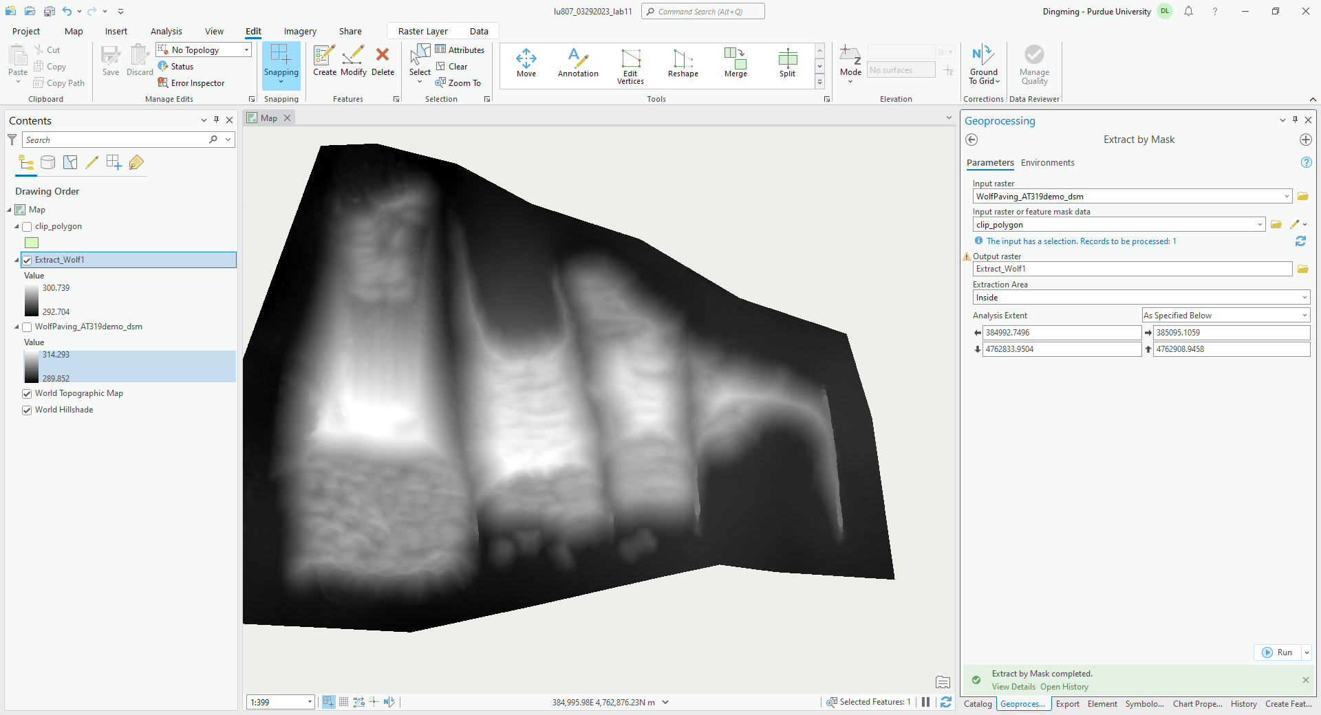
A. Extract by mask
- A new polygon layer was created in the same database. The polygon set the boundary of the bottom of the hill.
- Then apply the raster version of clip, it will keep the cells in the defined shape of combination of cells.
- Set input raster to the DSM data.
- Set feature mask data to the clipping shape.
- Rename the output.
B. Surface Volume
- Use “Surface Volume” to calculate the volume within an area.
- Set the input surface to the DSM.
- Set reference plane to above the plane.
- Click around the polygon to find the average elevation of the plane.
- Result was saved in a .txt file.
C. Map Creation
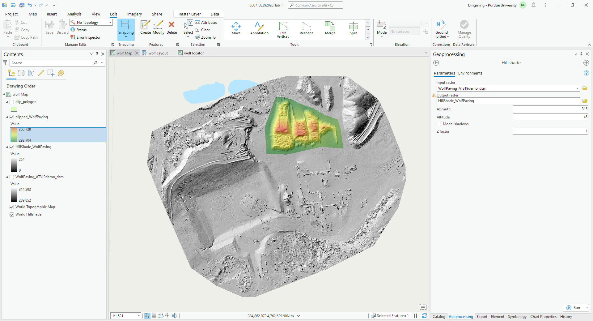
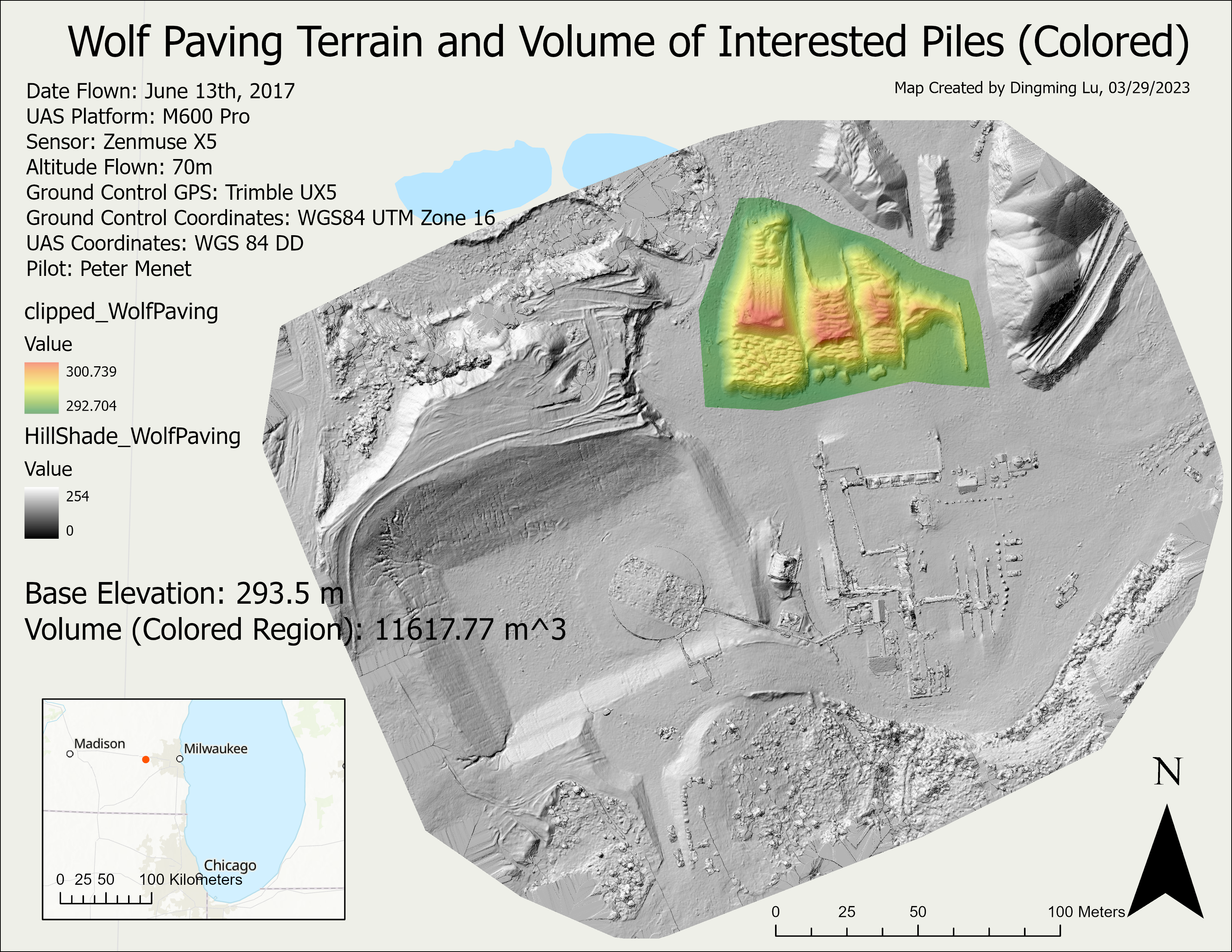
Create the hillshade, put on the metadata and other elements

III. Litchfield Analysis
- Same process was done on a second data set.
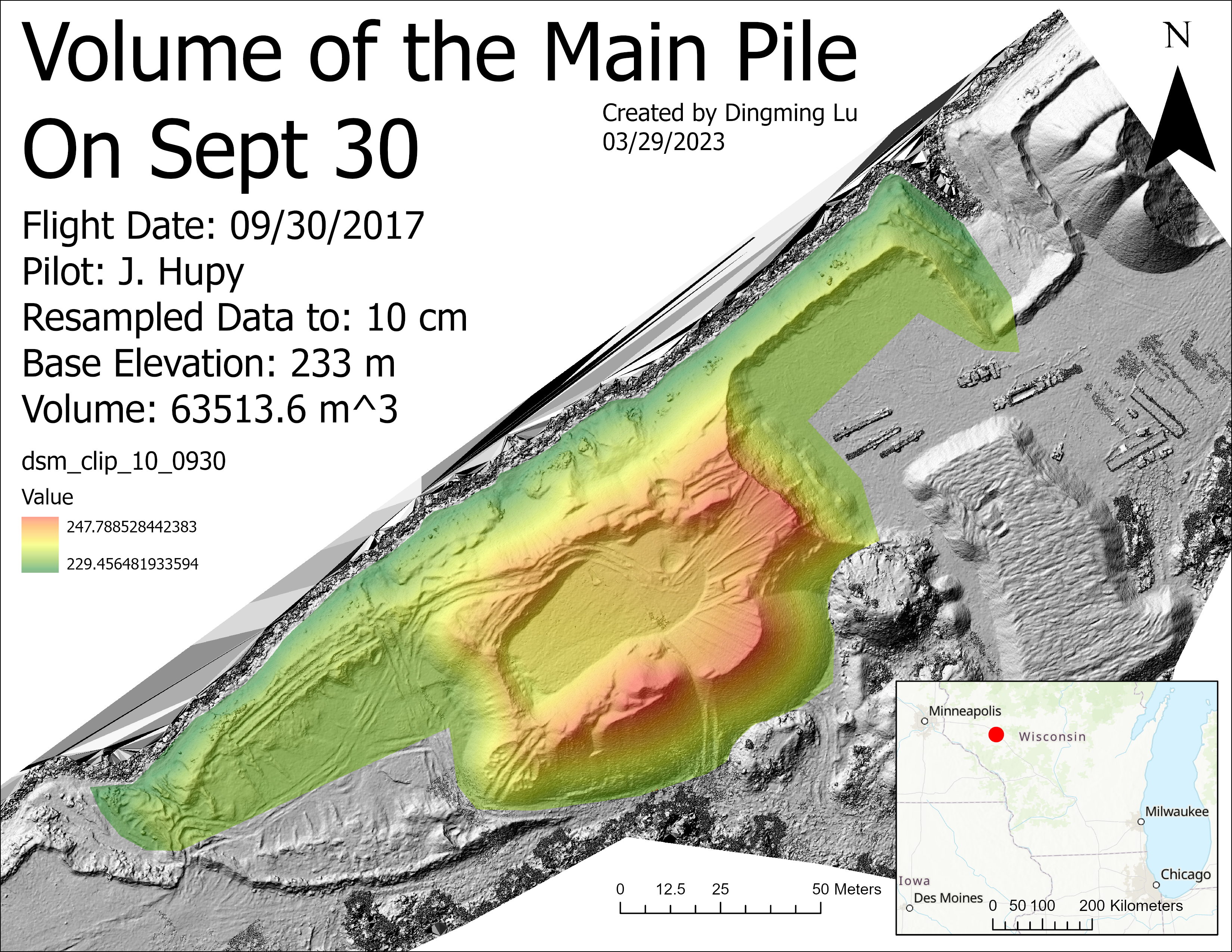
- Create polygon around the pile of interest -> extract by mask -> resample to 0.1m*0.1m and 1m*1m-> calculate volume -> create hillshade effect -> map
- Different resample size will produce different result.
- By changing the transparency and the appearance of the DSM data, we can overlay the DSM on to the hillshade layer and make it colorful.
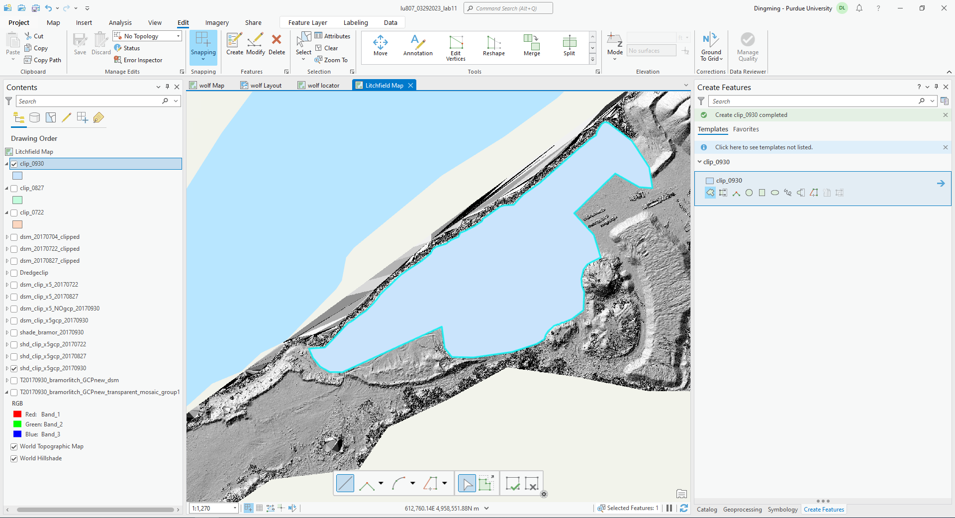
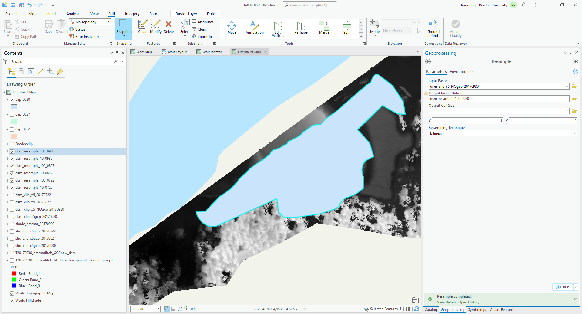
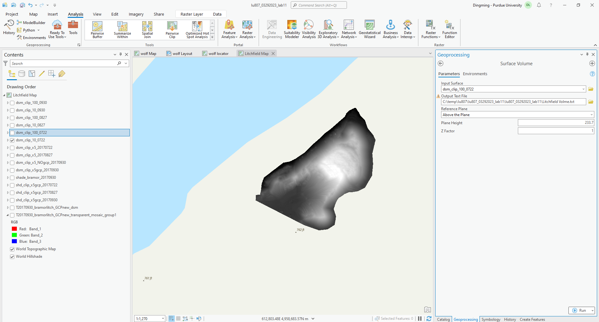
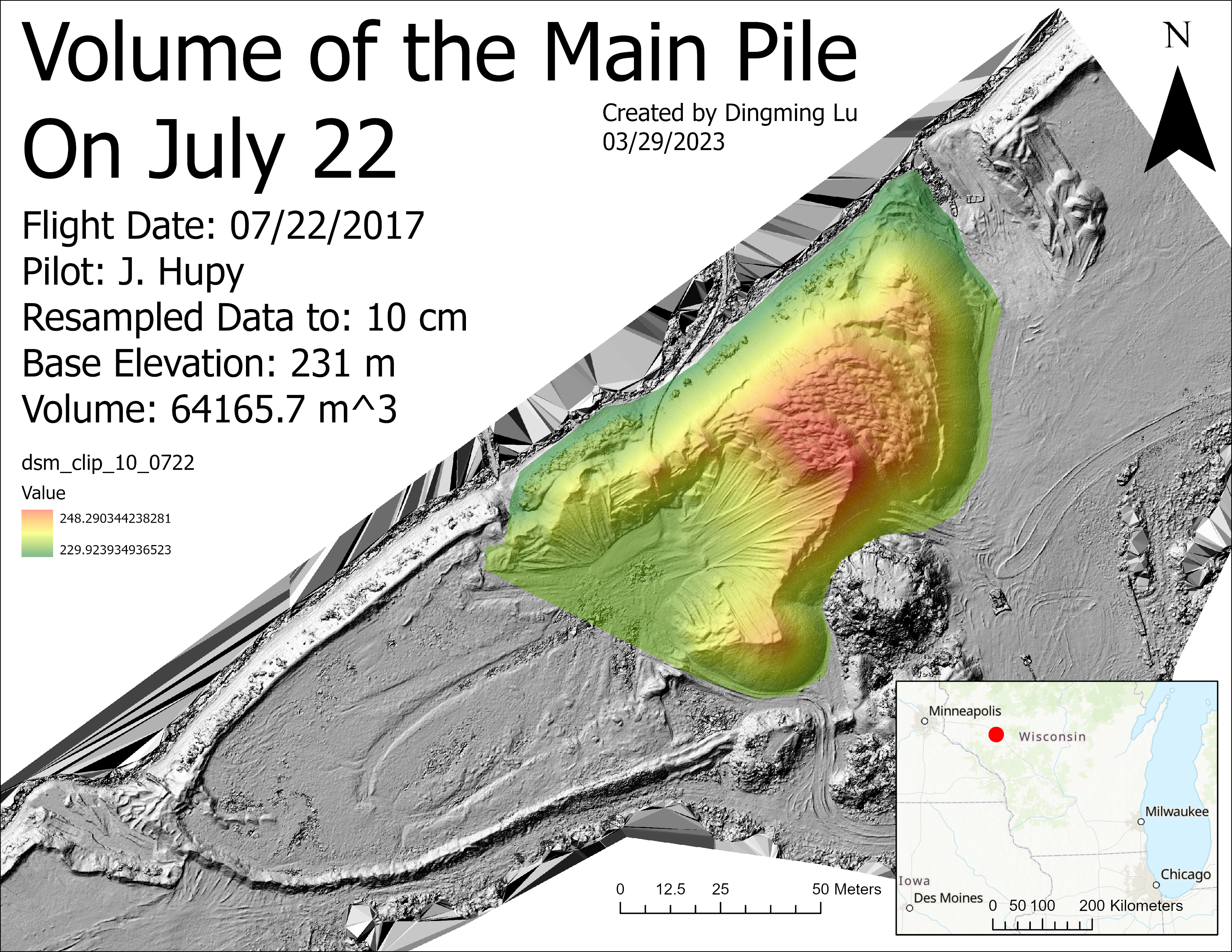
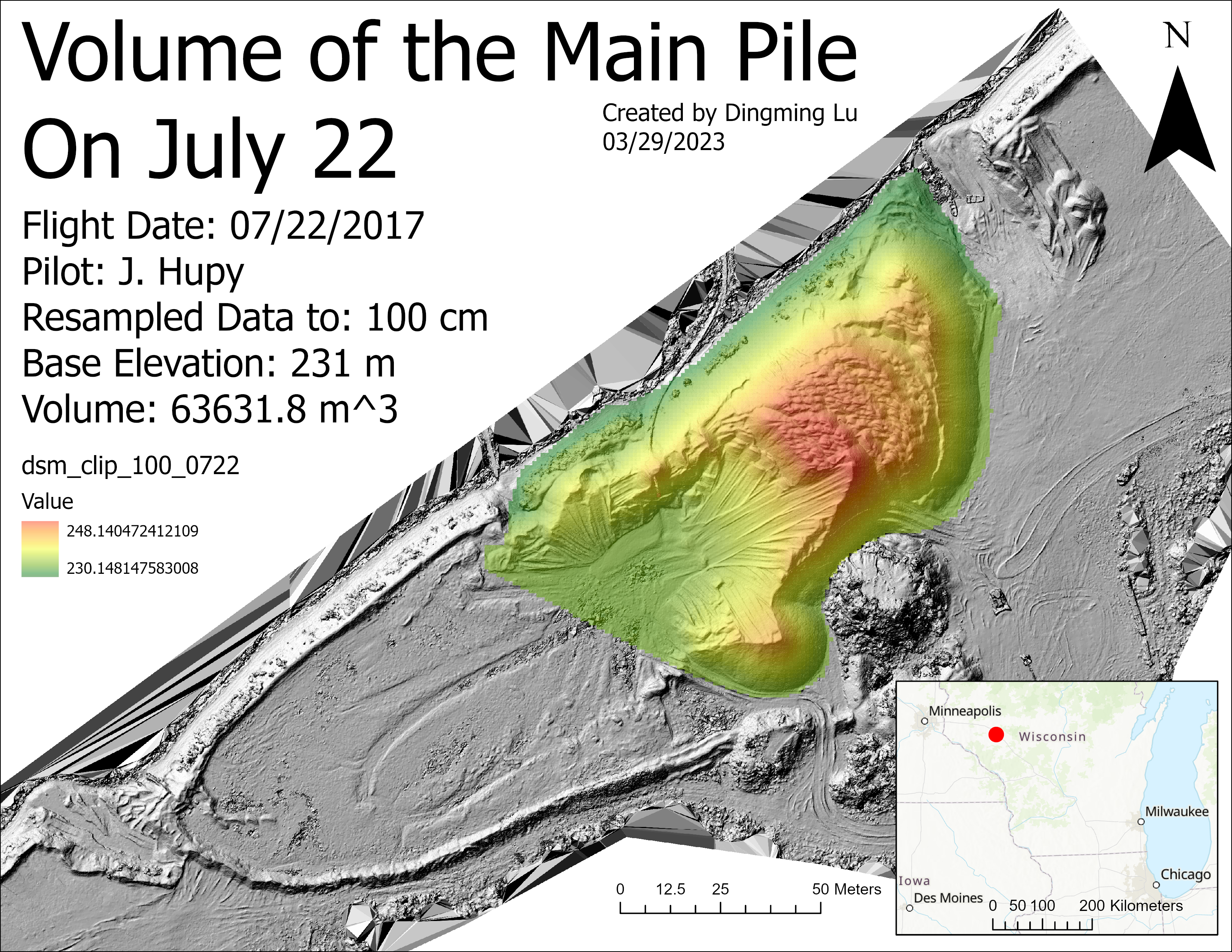
Figure 8 and 9: resampled to 10 cm. Right: resampled to 100 cm.
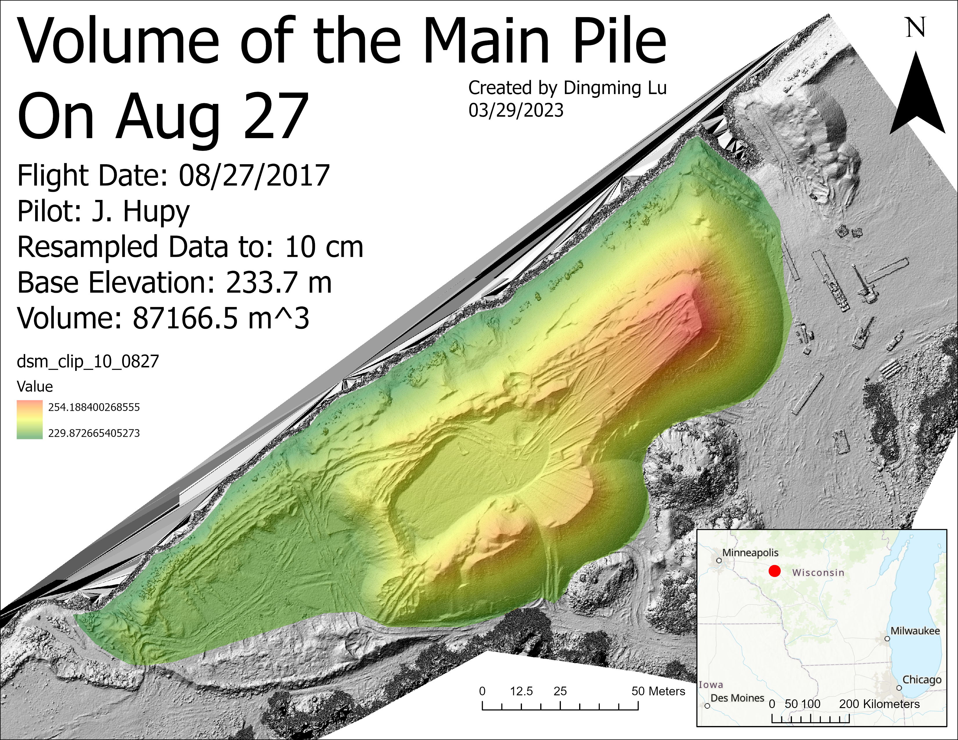


“Cut fill” was used to find the change of volume. It’s better to have a certain shape across the time.
